


CHAPTER A4 – DISCOUNT RATES
| CHAPTER A4 – DISCOUNT RATES | STATUS & REVISION HISTORY | ||
|---|---|---|
| Original Standard | May 1999 | NZIF April 2019 revisions:
|
| Review by Forestry Australia Valuation Working Group | Sept 2020 | Main revisions are:
|
| CURRENT STATUS | July 2025 | Released as final |
PDF available to download here
Introduction
Investment involves a commitment of funds for a period of time in order to derive a suite of future expected payments. Investors expect to earn a return in exchange for their commitment of funds. This is to compensate them for:
- The period of time the funds are committed;
- Expected inflation rates during the commitment period; and
- The uncertainty and risk associated with future cashflows.
Discount rates can be used to express the required rate of return, or compensation, that investors expect to receive in exchange for their commitment of funds. They are a fundamental component of Discounted Cash Flow (DCF) analysis and are one of the factors to which Net Present Value (NPV) based valuations are most sensitive.
Different discount rates may apply to the tree crop, land, carbon, roads and other durable assets. Each of these assets has unique features, the associated cashflows may have different levels of risk, and the market may have different required rates of return for each.
Discount rates and valuation approaches
Discount rates find expression in each of the main recommended approaches to valuation:
- within the sales comparison approach, a compelling unit of comparison to which sales can be distilled is the Implied Discount Rate (IDR);
- the income (or expectation) approach is a classic expression of DCF methodology. As such, it requires an explicit representation of discount rate; and
- Cost-based approaches to valuation may make use of compound rates. Compounding is the inverse of discounting and, as such, it also requires the selection of an appropriate rate.
The various roles for discount rates find widespread endorsement among forest valuers. There is less agreement on which individual rates to apply. Forest valuers typically consider a variety of sources and evidence when assessing, selecting and applying discount rates.
These may include:
- Cost of capital derivations – the cost of capital derivations may be based on asset pricing models such as the Capital Asset Pricing Model (CAPM) or Arbitrage Pricing Theory (APT) to derive an expected cost of equity. These may then be incorporated into Weighted Average Cost of Capital (WACC) models to reflect the cost of both equity and debt capital;
- Implied Discount Rates (IDRs) – such rates are derived from previous transactions. They are derived by constructing a cashflow for the comparable sale and finding the discount rate(s) at which the present value of the cashflow matches the transaction value;
- Applied or Declared Discount Rates – discount rates applied by the forest owner or independent forest valuers when valuing forest assets;
- Declared Hurdle Rates – hurdle rates represent the minimum threshold that an investor seeks to achieve on their investment;
- Capitalisation rates and multipliers – capitalisation rates and multipliers are commonly used in the property and real estate market. A range of rates is demonstrated, depending on the nature of the revenue to which they are applied. As a generalisation, such rates are applied to the average quantity generated in a single period, although variants allowing ongoing real growth and other adjustors are also demonstrated; and
- Internal Rate of Return (IRR) – as its name implies, the IRR is internal. There is near universal agreement within forest appraisers that this disqualifies its use in valuing the forest. DCF theory instead suggests that the rational purchaser of a forest must attend to the opportunity cost of their capital. The latter references external investment alternatives. The IRR can nevertheless figure in the evaluation process, especially when addressing the attractiveness of perpetuating the forest after the current rotation.
A further classification of rates
One means of classifying discount rates is to distinguish those constructed as ‘built-up’ rates versus those derived from empirical evidence. This might see the rates described above in the following classifications:
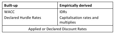
Such a classification must be applied warily. A key element within the WACC, for instance, is the so-called applied with the CAPM. This factor is derived from empirical market evidence.
The potential importance of the classification is that it distinguishes the genesis of the rates. This becomes important when there are attempts to merge rates from different sources, such as by averaging, or ‘reconciling’ the different estimates. The rates are not structural siblings in their derivation, even if they share a common intended purpose. Only so much reconciliation is possible.
Application of discount rates
Nominal or real
Nominal discount rates include the anticipated effects of inflation during the commitment period. Real discount rates exclude the effects of inflation.
Discount rates applied in forest investment analyses are most commonly expressed in real terms.
There are two main reasons for this:
- forest investment analyses may occupy long timeframes as even modest rates of inflation, numbers that are expressed in nominal terms may grow to unrecognisable levels thus denying the opportunity to readily check their credibility; and
- future levels of inflation are uncertain thus removing the need to include inflation relieves the valuer of one more uncertain assumption.
Forest valuers elect real cashflows mindfully. There are certainly circumstances where they will use nominal cashflows, or conduct both representations in parallel. Where there is a requirement to explicitly model debt servicing, nominal cashflows are more likely to be used. This is because the loan principal and repayments are fixed in historic terms. Similarly, rigorous modelling of the application of Australia and New Zealand’s current forestry taxation regime requires that the effects of inflation be addressed.
The conversion from nominal rates to real rates employs the Fisher* equation
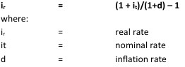
*Irving Fisher’s monograph Appreciation and Interest (1896) proposed this equation showing the relation between the nominal interest rate, the real interest rate and inflation. See https://archive.org/details/appreciationinte00fish
Cashflow timing conventions
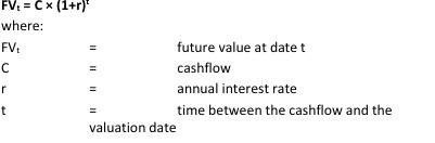
Valuing a series of cashflows that occur at different points in time is achieved by converting cashflows to the same point in time. This is achieved by either compounding or discounting. The future value of a present cashflow is derived via compounding:
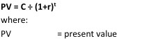
Conversely, the present value of a future cashflow is derived via discounting:
When compounding or discounting cashflows, different results will arise, depending on when cashflows are assumed to occur during a period. Modern computing capability and functionality means that there is little incremental effort in introducing precision to cashflow timing conventions.
For simplicity, valuers may assume that net cashflows arise (on average) at the midpoint of a cashflow period. If estimating the present value at 1 July of a cashflow occurring between 1 July to 30 June, the valuer may assume that the cashflow arises at the midpoint of this period, i.e. around 31 December. This timing implies that one-half of an annual period separates the cashflow from the valuation date and, as such, present value would be estimated assuming n = 0.5.
Estimates of future available cashflows are often comprised of concurrent forecasts of gross revenues (e.g. delivered log revenues), cost of goods sold (e.g. harvest, loading and delivery costs), operational expenditure (e.g. silvicultural and property management costs), capital expenditure (e.g. roading costs) and indirect and overhead costs. Depending on their anticipated timing, cashflows associated with particular cost and revenue streams can be compounded or discounted separately. An example of such an instance may be planting costs which are mainly incurred during the winter months in Australia’s southern states and New Zealand.
By default, many spreadsheet packages assume cashflows occur at the end of an annual period, e.g. Excel’s NPV function. In forest valuation, this generally leads to a conservative outcome. Careful examination of which cashflow timing convention might be applied is appropriate.
Cashflows
In conducting a DCF analysis using pre-tax cashflows, the revenue and cost streams must be just as the name implies – cash only. The exception to this may be the inclusion of a notional land rental, which may be included to apportion the NPV of future cashflows between the crop and the land. Capital Expenditure (CAPEX) should be modelled in the cashflow as and when it is expected to occur.
Outgoings such as depreciation or amortisation should be excluded. Pre-tax cashflows should not include interest servicing charges, since to include these may effectively represent discounting twice.
Leverage, as noted by Berk, DeMarzo, Harford, Ford and Finch (2011), refers to the extent to which a firm relies on debt as a source of financing. Debt may come in the form of (but is not necessarily limited to) bank debt issued by banking and lending institutions or debt-like instruments (e.g. promissory notes) issued by forestry investment vehicles to institutional investors who may have also made equity investments into these forestry investment vehicles. Leverage as it relates to this discussion includes all forms of debt and debt-like instruments, regardless of source.
In a levered post-tax cashflow model the effects of interest in reducing taxation (the so-called ‘interest shield’) can be included and interest payments deducted to give free cashflow. In an unlevered post-tax cashflow model interest payments are not deducted and no ‘interest shield’ is recognised. Both levered and unlevered post-tax cashflow models recognise the impact of depreciation and amortisation in reducing the amount of tax, but these notional items should not be recognised in the post-tax cashflow that is the subject of discounting.
The levered and unlevered cashflows are often referred to as:
- Levered Free Cash Flow (FCFE) or Free Cash Flow to Equity – levered post-tax cashflow; and
- Free Cash Flow to the Firm (FCFF) – unlevered post-tax cashflow.
It is important that cashflows are well defined, and that the discount rate applied to the cashflow has been derived in a manner appropriate to the cashflow to which it is applied.
Current rotation versus multiple rotation cashflows
Forest valuations prepared consistent with International Financial Reporting Standards (IFRS) for asset reporting purposes are guided by IFRS 13 (Fair Value). IFRS presents a similar overall target to contemporary valuation standards. In the absence of immediately comparable values, these encourage the valuer to follow the practices by which market participants arrive at an agreed transaction value.
Plantation forests
With plantation forests of sizeable scale, and where subsequent rotations are intended, most market participants are observed to prepare wood flow and cashflow projections on a multiple rotation basis.
Once the value of the plantation forest asset is identified, other IFRS standards specify that this value is to be apportioned between certain components. Two such components are the land value (specified under IAS16 – Property, Plant and Equipment) and the value of the current crop (IAS41 ¬– Agriculture). There is no clearly identified or straightforward location to declare the value associated with future rotations. This has generated some informed debate in the ranks of forest valuation clients and the forest valuers themselves.
In at least some quarters there has emerged reference to ‘IAS41 forest valuations’. This has been unfortunately misleading; it is clear from the expression of IAS41 that it is a reporting standard rather than a valuation standard and that its scope is confined to the current crop. It is not a standard for valuing complete forests – this role falls to IFRS13 and its cohorts from the valuation standards.
IFRS does not in any way insist that a plantation forest valuation must be based on just the current rotation cashflows. Despite this, other motivations may encourage such an approach. These are addressed elsewhere in these standards, but include inter alia concerns with the amount of conjecture required in estimating the performance of future rotations. As a result, there is an accumulated body of practice demonstrating valuations on both ‘current rotation’ and ‘multiple rotation’ bases.
While various options exist as to the selection of the appropriate cashflow to be used for valuation purposes, there is a singular fair value for the forest estate.
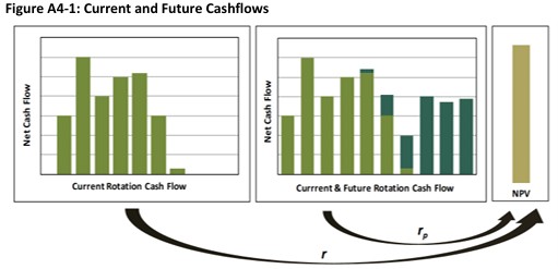
Referring to Figure A4-1:
- For convenience, the series of revenues flowing from the plantation forest are all shown to be positive;
- For the one NPV result, two possible representations of the responsible cashflows are presented. The first is based on the cashflows associated with the current (existing) rotation, whereas the other corresponds to those associated with continued management of the forest; and for each of the cashflow versions there is a corresponding discount rate, illustrated as r and rp respectively, that give rises to an equivalent NPV. There is no single and universal adjustment between the discount rates. The differential between the rates may be influenced by a variety of factors, but in particular the rate of return generated by re-investment in forestry and the treatment of land.
Natural forests
With natural forest management, current and future rotations may be undefined in situations where harvest and silviculture regimes result in or maintain a multi-age class structure.
Examples of natural forest management regimes include:
- block clearfell used in even-age single species forest types. Variations may include leaving a widely spaced even distribution of seed trees for re-seeding;
- Australian Group selection (remove dominant plus surrounding trees) used in uneven-aged, multiple species forest types. Variations may include shelterwood silvicultural systems.
- single tree selection used in uneven-aged, multiple species forest types; and
- thinning from below or above to reduce stocking and promote growth.
In situations where the transition modelling from current to future rotations is practically infeasible (transitioning taking place at the individual tree level rather than the stand level), an appropriate discount rate should be applied to the cash flows associated with the harvesting of the existing forest, reportable under IAS41 ¬– Agriculture.
In determining the periodic (annual) allowable cut for long-term planning, forest recruitment and regeneration should be considered.
Multiple cashflows and multiple discount rates
The differentiation between cashflows associated with current rotations versus investment models, and more recently those associated with the purchase and/or sale of carbon – in Australia under the Emissions Reduction Fund (ERF) or in New Zealand under the Emissions Trading Scheme (ETS), emphasises the point that multiple discount rates may be applied and assumed as part of forest valuations.
An example is the case where the carbon trading opportunity is being valued.
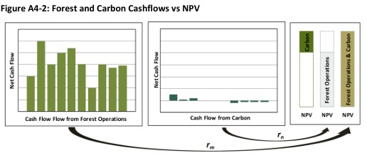
Referring to Figure A4-2:
- the discount rates applied to a set of cashflows associated with forest operations and those associated with carbon may differ; and
- For each of the cashflow versions there is a corresponding discount rate, illustrated as rm and rn respectively – the derivation of each discount rate may be completed independently.
Pre-tax and post-tax cashflows
This aspect of discount rate terminology provides opportunity for confusion. A ‘pre-tax discount rate’, for instance, would generally be understood to imply a rate that ignores taxation effects. This rate will be applied to cashflows that similarly avoid any inclusion of taxation (the so-called pre-tax cashflows).
To some observers a ‘post-tax rate’ is that rate which would be applied to cashflows that explicitly recognise and net out taxation (post-tax cashflows). It is therefore a discount rate that is applied to ‘post-tax’ cashflows. To other observers, a ‘post-tax’ rate includes adjustment for the effect of taxation. When applied to pre-tax cashflows it is intended to provide the same result.
It is important, therefore, that the valuation commentary explains quite clearly just which rate is being used. The terms pre-tax and post-tax should not be applied to discount rates but rather to the cashflows modelled. The preferred terminology is that pre-tax cashflows ignore taxation effects, while in deriving post-tax cashflows taxation effects are explicitly modelled.
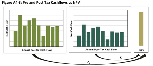
Referring to Figure A4-3:
- by discounting the cashflows the valuer arrives at the NPV of the forest, represented by the single block of value applying at the time of valuation;
- as explained in Chapter B12 of these Standards (Forest Valuation Method), in any attempt to estimate market value the valuer is trying to anticipate the price at which a forest would actually and willingly change hands in a fair transaction – there can only be one such value as the purchaser writes only one figure on their cheque);
- for the one NPV result two possible representations of the responsible cashflows are given below – the first (a) does not net off taxation obligations (the so-called pre-tax cashflow), whereas the other (b) does (the so-called post tax cashflow); and
- for each of the cashflows represented there is a corresponding discount rate, illustrated as rs and rt respectively, that will give the same NPV – I n the case illustrated, rt will clearly be less than rs in order to derive the same fair value.
Which tax rate?
Construction of a post-tax model requires assumptions to be made about what tax rate to use. Possible alternatives for the marginal tax rate are:
- model the personal tax circumstances for potential individual purchasers whose tax status is known; or
- create a generalised construct for potential purchasers.
Modelling individual circumstances represents a more rigorous approach and, in some cases, may be appropriate ¬– we might expect that those with the least tax burden would be able to pay the most for a forest. Of course, if the best-positioned purchasers are commercially astute, they will not pay more for the asset than they need to in order to see off their competitors.
The generalised model may be adopted, but with the expectation that a careful forest valuer will identify where deviations might be expected. Two extremes could be where:
- the market may be set by active competition between buyers whose tax exposure is low; and
- the only likely participants may be those whose taxation exposure is comparatively high. Some offshore buyers, for instance, may not be able to fully exploit the safe harbour offered by related party debt due to unfavourable home country tax rates.
These standards acknowledge that at some levels of the market individual investors and their personal taxes may need to be recognised. A generalised taxation construct that establishes the assumed circumstances of a notional set of corporate and individual investors might be adopted to enable the preparation of ‘base case’ valuations. The procedure is further described in Chapters A5 and B11.
Pre- or post-funding (capital structure)
The capital structure assumed in a forest valuation will affect the NPV. In common with the pre-tax/post-tax position outlined above, the amount of equity, internal debt (e.g. corporate bonds), related party debt and external debt (e.g. third party bank debt) assumed in the total forest funding package interacts with both the tax position (the tax treatment of borrowings and equity differs markedly) and the appropriate valuation discount rates.
A number of recent forest transactions have demonstrated the application of comprehensive affordability models. These have been prepared by both the vendors and purchasers party to these transactions. The models are generally based on a leveraged post-tax cashflow basis. There is careful attention to the free cashflow with which to service borrowing. Any such model cannot ignore the expenditure imposition arising from the re-establishment of the next and succeeding rotations or the timing of capital expenditure required to bring the trees to market. Commonly such a consolidated model is called an Enterprise Model or Purchase Model.
Within such models the purchasers of large forest estates in Australia and New Zealand typically structure the ownership and financing of the enterprise in a manner that is most tax efficient for their circumstances. A thin-capitalisation financing structure is commonly utilised by foreign investment in Australia and New Zealand by way of a related party loan to achieve a tax efficient structure.
Australia
The current Australian company tax rate is 27.5% to 30% of net profit before tax. Interest charged on debt is tax deductible subject to thin capitalisation restrictions. Under Australia’s current thin capitalisation restrictions, a ‘safe harbour’ debt level of up to 60% of assets (reduced by certain non-debt liabilities) is permissible. This broadly equates to a debt to equity ratio of 1.5 to 1.
Related party loans can provide tax efficiencies for investors as Non-Resident Withholding Tax (NRWT) is charged in Australia on interest payments at 10% compared with the Australian company tax rate of 27.5% to 30%. Franked dividends are exempt from NRWT, while unfranked dividends would typically be taxed at a rate of 5-30%, depending on the source of capital and relevant tax treaties.
New Zealand
The current New Zealand corporate tax rate is 28% on net profit. Interest charged on debt is tax deductible. Under New Zealand’s current thin capitalisation regulations, a ‘safe harbour’ debt-to-asset ratio of up to 60% is permissible. Related party loans provided from a safe harbour can provide tax efficiencies for investors as Non-Resident Withholding Tax (NRWT), charged in New Zealand on interest payments at 10-15%, depending on where the related party loan is domiciled. NRWT charged on franked dividends are exempt, while unfranked dividends would typically be taxed at a rate of 5-15% (or more), depending on the source of capital and relevant tax treaties.
A generic representation of thin capitalisation could be used by forest valuers to represent leverage in their representation of the post-tax cashflows associated with the valuation of ‘large’ forest estates. In this representation, although all sources of acquisition capital are ultimately provided by the shareholders of the enterprise, 60% of the funds could be considered debt for the purposes of capital structure and interest deductibility. The interest rate set on the related party loan must be ‘fair and reasonable’ and represent an arm’s length interest rate. Within such a model the debt-to-asset ratio must be monitored on an annual basis to ensure that the capital structure remains in compliance with thin capitalisation restrictions. In particular, to remain in compliance with thin capitalisation requirements, the model would generally need to reflect a reduction in debt levels over time as the standing timber is harvested and asset base diminishes.
A comprehensive model of this nature needs to incorporate estimates of the cost of standing timber deduction (Australia) or cost of bush depletion (New Zealand) and tax treatments. Given this, models of this nature are often formulated in nominal terms.
Increasing debt levels may raise the expected profitability of the project but can increase its risk. The risk must be reflected in the discount rate applied to the project, and an appropriate method of reflecting interest on the debt and debt repayment should be included.
Adoption of a model that assumes 100% equity funding and uses a post-tax approach that only includes the tax effects related to full equity funding (see Chapter A6) may, in some cases, provide for an appropriate starting point for a post tax cashflow construct.
It is noted that investors may use a number of different investment structures including trust structures (in particular to hold the forest and land assets).
Review of discount rate approaches
Cost of capital derivations and the weighted average cost of capital
Cost of capital derivations are typically based on asset pricing models, such as the Capital Asset Pricing Model (CAPM) or Arbitrage Pricing Theory (APT,) to derive an expected cost of equity. Cost of equity derivations can then be incorporated within Weighted Average Cost of Capital (WACC) models, along with the cost of debt, to reflect the blended cost of both equity and debt capital. Such derivations are extensively addressed in corporate finance literature, e.g. Berk et al. (2011), Reilly and Brown (2012) and Brealey et al. (2014). Readers are referred to such literature for further detail.
In its simplest manifestation, the cost of equity capital is multiplied by the assumed proportion of equity financing, and the cost of debt is likewise multiplied by the assumed proportion of debt financing. The results are added to give a composite rate. Adjustments have variously been applied to recognise attributes such as tax and liquidity.
Cost of equity
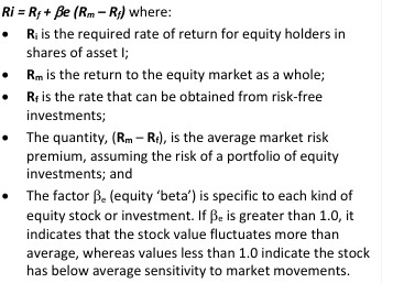
The framework most commonly used to estimate the cost of equity is the CAPM, which is used to estimate the required rate of return for an asset given its non-diversifiable (systematic) risk. When applied to equity capital the CAPM states:
Risk-free rate (Rƒ)
The risk-free rate is the rate of return attributable to an investment with no risk of financial loss. In practice, Government bond rates are used as a proxy for risk-free rates. Gresham (1993) argues that since, in theoretical terms, the CAPM is a single period model, the short-term Government bond rate appears appropriate. However, he also concedes that since forestry is by nature a long-term investment, the long-term rate may be more applicable.
Beta (β)
β is a measure of the systematic risk of an entity, i.e. the non-diversifiable risk or that part of the risk of an asset that cannot be diversified away. β represents the tendency of a security’s returns to respond to movement in the market as a whole. β is calculated by dividing the covariance of the security’s returns and the benchmark’s returns by the variance of the benchmark’s returns over a specified period.
A key feature of β that deserves discussion is that given information on the market as a whole, and the trend in a particular stock price, can be derived with authority and precision. Different practitioners will get the same result. This escalates its attractiveness – it is a comparatively objective measure. Where professional opinion and insights come into play, however, is in understanding why certain stocks might behave differently and which ones might not belong in the pool.
Expression of β is not without complication, as β s may be specified on either an ‘asset’ basis (i.e. the total investment in the asset) or for just the ‘equity’ component of the investment. The more debt an entity has in its capital structure, the higher the levered or equity β of the entity. Synonyms for these terms are ‘unlevered β ’ and ‘levered β ’ respectively.
Conversion between the two forms is provided by the equation:
Asset β = equity β /(1 + (1 – tax rate)* debt/equity)
Use of CAPM analysis in forest investment valuation has encouraged various attempts to identify an appropriate β . Market information associated with pure-play publicly listed forest investment companies provides for the most authoritative source of statistics from which to derive β . However, the progressive shift in forest ownership from publicly held vertically integrated forest product companies* and pure-play forest investment companies towards institutional ownership has led to a paucity of information from which to derive betas in an Australasian context. Betas by industry sector are regularly compiled and published by corporate finance professionals such as Aswath Damodaran*. A review of β s published in January 2015 incorporated estimates for 42,410 global firms, only 303 (0.7%) of which related to the paper and forest products sectors (Damodaran, 2015). A detailed review of the firms included revealed the existence of virtually no comparable pure-play forestry firms from which βs could be derived for Australasia.
*Market statistics associated with vertically-integrated forest product companies represent a less than perfect source of
information from which to derive β for pure-play forest investments. The various parts of the integrated business might display
differing market correlations and the β associated with the integrated business will therefore differ from that of pure-play
forest investment.
*See http://people.stern.nyu.edu/adamodar/
Alternate approaches have used US data to derive betas, or estimate betas from the Security Market Line using expected returns derived from timberland indices incorporated within NCREIF (National Council of Real Estate Investment Fiduciaries) (Reilly & Brown, 2012). These have then been used with US risk-free rates and risk premia to derive US CAPM, which have then been adjusted to incorporate geographically derived risk premia.
Given the above, the resulting range of β estimates derived and disclosed in Australasian forest valuations over recent years has been broad.
The estimation of an appropriate β has invariably required valuers to exercise their professional judgement. Factors which impact on the β include, but are not necessarily limited to:
- nature of the industry;
- duration of contracts;
- type of customer;
- industry regulation;
- presence of real options;
- operating leverage; and
- market weight.
Market risk premium (Rm -Rƒ)
Market risk is non-diversifiable (systematic) component of the total risk on a specific investment an investor may face. The other component is diversifiable (non-systematic) risk.
Market risk describes how returns on an investment tend to move with the market as a whole. Some correlation is to be expected, since individual investments are likely to show some common response to such factors as interest rate changes, general price level changes and fluctuations in economic growth rate.
Diversifiable risk defines that proportion of the total risk which is peculiar to a particular investment. Examples in forestry could include fire and wind damage, insufficient log value recovery at harvesting, or unforeseen restrictions on harvesting. Investors cannot expect to be rewarded for taking on non-systematic risk as it can be diversified away.
Portfolio analysis has demonstrated that non-systematic risks can be eliminated through the construction of a diversified portfolio of securities. Conversely, diversifying the portfolio offers no escape from systematic (market) risk, which is embodied in all investments. The CAPM is concerned with non-diversifiable (systematic) risk. An asset’s β is a measure of the non-diversifiable risk of the asset relative to the risk of the market.
Equity cost of capital
To derive the equity cost of capital for an unlevered asset using the CAPM leads to calculations such as the following (example only):
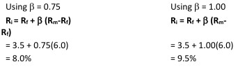
The example assumes a risk-free rate of 3.5% and a market risk premium of 6%. The rates in this example include inflation. The effect of adjustment for an inflation rate of 2.5% gives a real cost of capital in the range of 5.4% to 7.1%.
Cost of debt
The cost of debt is the cost of funds attributable to the risk of the company’s assets if the funds were borrowed on a non-recourse basis. The cost of debt will be at a premium to the Treasury or Government bond rates (Marsden, 2009).
Weighted average cost of capital
The WACC reflects the blended cost of both equity and debt capital. Subsequent to an estimation of each of the cost of equity and cost of debt, the WACC can be determined according to this formula:
WACC = (E/(D+E))R+ (D/(D+E))Rd(1-t)
where:
• E is the value of equity
• D is the value of debt • Ri is the cost of equity
• Rd is the cost of debt
• t is the corporate tax rate.
Assuming a cost of equity of 8.0%, a cost of debt of 5.0%, a debt-to-value ratio of 20% and a corporate tax rate of 28%, the WACC can be derived as follows:
WACC = (0.80) x 8.0%+ (0.20) x 5.0% x (1-28%)
= 7.12%
The rates in this example include inflation, and the resultant WACC is a nominal rate for application to nominal cashflows. WACC is typically applied to nominal post-tax cashflows – the so-called free cashflow to the firm*.
In the example given, the effect of adjustment for an inflation rate of 2.5% gives a real adjusted WACC of 5.56% for application to real post-tax cashflows.
*Free Cash Flow to the Firm (FCFF) – cash distributions available to both debt holders and equity holders after all
expenses, taxes, asset maintenance and reinvestment.
Limitations associated with WACC derivations
A variety of complexities exist which make the application of WACC-based derivations to forestry cashflows challenging. The WACC formulation presented above requires corporate tax be deducted. For forestry assets, this assumption can be too simplistic.
Specific to forest investments in New Zealand and Australia, the tax shield offered by the ‘Cost of Bush’ (New Zealand) and the ‘Cost of Standing Timber Deduction’ (Australia) means that the tax payable on income is close to 0% at acquisition where there is immediate harvest. However, the tax payable trends toward the corporate statutory rate over time as the ‘Cost of Standing Timber Deduction’ is depleted through harvest activities.
Furthermore, the actual post-tax position of a firm can be influenced by a variety of factors including asset specific tax rulings, the use of both internal and external debt, and changes in debt-to-equity ratios (capital structure) through time. The collective impact of these variables may make determination of the value of an asset difficult to estimate under a DCF valuation model. This is partly because of the relatively simplistic manner in which equity and debt are combined into the WACC. Damodaran (2006) notes that the exercise becomes increasingly complex as debt ratios change over time.
Given that the corporate rate can vary by entity and through time, applying the full corporate tax rate can result in an inappropriate estimation of the WACC to be applied in a forest valuation.
While limitations and challenges exist with deriving discount rates using cost of capital-based derivations, this is not to imply that such approaches be abandoned. Rather, that forest valuers remain cognisant of such complexities, and exercise caution and discipline when deriving discount rates using a cost of capital approach.
Implied discount rates
The IDR is a particularly useful metric which can be extracted from forest transactions. Its use can represent a sales comparison approach to valuation within a DCF construct. Derivation of the IDR involves the development of a credible cashflow projection for the transacted forest. The discount rate at which the DCFs match the purchase price is the IDR.
Given the heterogeneity of forest assets, a comparable sales approach using an IDR is often more credible than simpler attempts at comparisons based on factors such as $ per hectare.
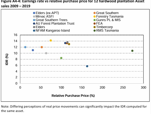
A significant restructuring of Australia’s hardwood plantation assets occurred during the period 2009 to 2019, initially triggered by the collapse of many management investment scheme (MIS) companies. Margules Groome, a forestry consulting firm, examined the announced sales prices in the context of information memoranda and other data at its disposal. This analysis work suggests that a possible range of implied discount rates can be demonstrated over the ten-year period. The correlation between relative sale prices and IDR appear to be weak. Variables as perceived by investors such as the level of distress, the outlook for Asian hardwood woodchip markets, foreign exchange and freight rates likely significantly influenced sales prices (Figure A4-4).
Figure A4-4: Earnings rate vs relative purchase price for 12 hardwood plantation Asset sales 2009 – 2019
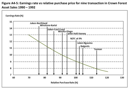
The New Zealand Crown Forest Asset sales programme involved some 350,000 ha of plantation forest which was sold to private enterprise in 13 units over the period 1990-1992. Chandler Fraser Keating, a forestry consulting firm, examined the announced sales prices in the context of information memoranda provided by the Crown prior to the sale. Using their own estimates of log sale prices, they concluded that a range of discount rates had been demonstrated in Figure A4-5 (Keating, 1990).
Figure A4-5: Earnings rate vs relative purchase price for nine transaction in Crown Forest Asset Sales 1990 – 1992
Two members of the Crown Forest Asset Sales team published an analysis of the sale results (Manley & Bell, 1992). They explored four different models which incorporated the major variables that might be expected to influence forest value. The discount rate is treated as a solution variable. The two models which most effectively explain the variation in forest values are in Table A4-1.
Table A4-1: Discount rates for Crown Forest Asset Sales estimated by Manley and Bell (1992)
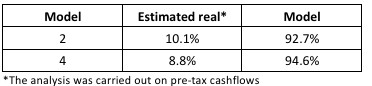
After recognising standard errors associated with the estimates, Manley and Bell (1992) concluded from Model 2, that ‘… [the] estimates imply that real pre-tax discount rates in the order of 9 11% were used in valuation of the State plantations. These estimates of discount rate are linked to the rotation age assumed and level of prices assigned’.
IDRs derived by forest valuers have been historically published in Manley’s biennial discount rate surveys (Manley, 1998, 1999, 2001, 2003, 2005, 2007, 2010, 2012, 2014, 2016, 2018, 2020). Historic IDRs derived by forest valuers for New Zealand and Australian transactions are presented in Figure A4-6.
Figure A4-6: IDRs (applied to current rotation pre-tax cashflows) for transactions reported in each of the discount rate surveys. Forests are identified by size class (small <1000 ha; medium 1000 to 10,000 ha; large >10,000 ha).
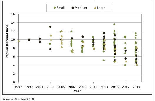
IDRs require very careful interpretation. The cashflow representation from which an IDR is derived is totally at the valuer’s discretion. Discretionary choices include: current rotation, perpetual model, pre-tax cashflow or post-tax cashflow, log price and log price growth, wood flow assumptions etc.
In addition, not all IDRs are created equal:
- some IDRs are derived from a comprehensive analysis of transaction and associated cashflows;
- others are derived from a crude representation of cashflows; and
- others might have been lifted from discount rates reported in company accounts associated with a forest asset prior to a transaction occurring.
The selection of the appropriate IDR to apply to the subject cashflow needs to be drawn from IDRs associated with transactions that share similar characteristics with the subject forest, and that have been derived using a methodology consistent with the manner in which the IDR is to be applied.
More recent discount rate surveys (e.g. Manley, 2019) have been updated to allow for the separate reporting of IDRs applied to the current rotation and multiple rotation cashflows. Recognition of the existence of multiple IDRs assists in reconciling the various sources. The impact of forest size on discount rate has also been recognised.
Applied or declared discount rates
Discount rates employed in asset reporting
At the time of writing, publicly reported companies in Australasia have declared that the rates in Table A4-2 have been used in valuing their forest assets.
Table A4-2: Discount rates declared in financial reporting for Australasia-registered companies with annual reports in the public domain are shown in the table below (all rates are applied to real current rotation pre-tax cashflows)
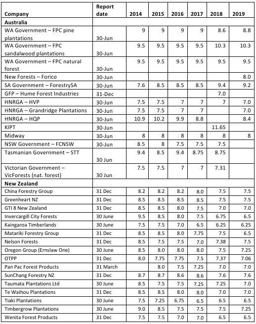
Varying levels of disclosure concerning the valuation methodology and critical assumptions employed are reported in the company accounts. The level of disclosure covers the spectrum from little through to a relatively unambiguous and high level of disclosure.
Many of the disclosures made in the company accounts listed above assert that the asset has been valued on a ‘going concern’ basis. In most of these cases, while the asset may have been modelled on this basis the valuation has been confined to the current rotation cashflows. The reported discount rate pertains to just this portion of the ‘going concern’ cashflow.
For many readers valuation on a ‘going concern’ basis suggests the use of full operational or enterprise cashflows that include reinvestment in the asset base through ongoing reestablishment activities and the subsequent realisation of harvest revenues from these activities. Such ambiguity can lead readers to misconstrue that the discount rate used by forest valuer in valuing the tree crop represents a measure of the return on investment from the enterprise.
Despite the preparation of the company accounts by parties other than the forest valuer, it is incumbent upon the forest valuer to ensure unambiguous disclosure around the derivation of the tree crop and forest asset values.
Disclosure of applied discount rates
A framework for the preferred level of discount rate(s) and associated valuation disclosures is set out below. Disclosure regarding such characteristics as the following afford forest valuers an improved basis on which they can assess discount rate evidence:
- The various discount rate(s) employed in valuing the assets and the specific asset value that were used in deriving them, e.g.
− an estimate of tree crop value using a current rotation cashflow model;
− an estimate of forest estate value using an investment/ purchase model; and
− an estimate of carbon value; - The cashflows to which each of the discount rates were applied including:
− whether discount rates apply to nominal or real cashflows;
− whether the cashflows were on a pre-tax or post-corporate tax basis; and
− whether the cashflows include an explicit treatment of debt financing; - The methodology and treatment used to recognise freehold land;
- The presence or absence of lessee of lessor interests where land is rented; and
− a summary of key valuation assumptions including:
− harvest profile and markets; and
− a description of log prices employed in the valuation
Such levels of disclosure are fundamental in ensuring that discount rates drawn from different sources can be compared and applied appropriately.
Declared hurdle rates
Hurdle rates are primarily intended for use in investment decision making. The declaration of such rates does not necessarily imply their suitability for forest valuation as they may not represent the market perception of the desirability of a forest investment.
State-owned forests in Australasia previously provided a useful source of hurdle rates. The privatisation of these estates is nearly complete. With a high proportion of these estates now under private ownership, publicly declared hurdle rates have been scarce. Increased competition for capital to invest in forestry along with a scarcity of quality opportunities within which to deploy the capital raised has led Timber Investment Management Organisations (TIMOs) to be more circumspect in disclosing hurdle rates.
Despite the above, sporadic information does becomes available in the public domain. It can provide a useful benchmark for investor return expectations from investment in forestry.
Capitalisation rates and multipliers
Capitalisation rates are widely represented in the analysis of real estate investments, and in other real asset classes.
They are aligned with what the forest valuers refer to as discount rates, effectively being a subset of them. The distinction comes about because of their derivation and application. They are (mostly) based on the presumption of an equal annual earnings stream, such as is offered by the rent paid by a tenant. Because of the expectation of the even income flow, just one year’s average income suffices for both the derivation of the rate and its application.
The rates are derived from market evidence and, as such, they are more aligned with IDRs than with WACC-derived or ‘built-up’ rates.
Just as with IDRs, it is necessary to address the nature of the rental stream, including whether it is the rent before or after inducements offered to the tenant, occupancy rate, review mechanisms etc.
Potential application of capitalisation rates
Capitalisation rates from real estate activity are not sufficient for direct application in forest valuations. However, they may deserve closer attention for the following:
- as an expression of wider investment market buoyancy;
- as a confirmation of the level of variability that can be encountered within other asset classes; as evidence of the differences that are evident between sub-classes of real estate;
- identification of influences on investor perception from markets with abundant evidence;
- evident trends;
- the opportunity cost to diversified investors of taking funds out of real estate and putting it in timberland;
- the beta characteristics of other forms of real estate compared to timberland; and
- the importance in defining the rent and purchase price consistently.
Example sources of capitalisation rates: www.cbre.com.au/researchreports/Asia-Pacific-Cap-Rate-Survey-May-2020
Internal rate of return
There is general agreement that a forest project’s own IRR is an inappropriate basis for its valuation. Since it is by definition an internal rate, it does not address the investor’s alternate investment opportunities.
However, a market rate of return might be found from the minimum market acceptable IRR observed in a range of alternative forest projects. For example, offering documents for forestry schemes generally report an expected IRR. The offering documents generally give prominence to this parameter, and it could be concluded that their successful subscription demonstrates that the quoted IRRs either match or exceed the investors’ required return on equity.
Discount rate surveys
A limited number of surveys are periodically compiled on timberland discount rates. Such surveys include those compiled by the James W. Sewall Company (www.sewall.com), IWC (www.iwc.dk) and Professor Bruce Manley of the University of Canterbury. These surveys typically seek to disclose discount rates relating to certain forest assets derived using one or a number of the approaches previously discussed.
The discount rate surveys compiled by the James W. Sewall Company are prepared internally and are typically made available to clients using them for appraisal work. The surveys compiled by the International Woodland Company typically report rates that are publicly disclosed.
Since the second quarter of 1997, Manley’s biennial discount rate surveys have been published in the New Zealand Journal of Forestry. It is the most widely recognised survey referenced in Australia and New Zealand forest valuations and represents one of the most compelling tools at a forest valuer’s disposal. Forest valuers employed by forestry companies and consulting firms are surveyed on the discount rates that they employ in valuing forests.
The extent of the questions included in the survey has increased through time, with Manley’s most recent 2017 survey (Manley, 2018) asking the following questions:
- What methods do you use to determine the market value of a tree crop (or forest)?
- When using the income (expectation value) approach, what real discount rate do you use to estimate the market value of a tree crop (or forest)?
- What is the basis for deriving this rate?
- How do you determine the log prices used?
- How do you account for the cost of the use of land in valuing a tree crop?
- Do you include cashflows from only the current crop?
- When do you assume that cashflows occur?
- Do you apply a stand-based or estate-based approach?
- What specific allowance do you make for risk? Do you adjust the discount rate for forest-specific risk?
- What method do you use to determine the market value of the carbon trading opportunity?
- What real discount rate do you use to estimate the market value of the carbon trading opportunity?
- How do you determine the carbon prices used?
- What carbon trading strategy is assumed?
- How do you account for the cost of the use of land in valuing carbon?
- What is your estimate of the discount rate implicit in the transaction price of recent forest sales in New Zealand and Australia
- What real discount rate do you use to evaluate replanting or new planting investments?
- What is your estimate of the IRR on replanting or new planting?
The increasing level of disclosures and background relating to the discount rates generated through these surveys provides an improving base from which to interpret and analyse these data.
The results of Manley’s biennial surveys are summarised in Implied Discount Rate Section.
Risk and the discount rate
Sources of risk and uncertainty associated with forestry include:
- catastrophic events: For example, forest fires, windthrow, volcanic activity etc;
- other attrition: For example, disease, snow damage, browsing damage, landslides etc;
- growth performance: The closer to maturity the forest is, the less the uncertainty. However, at any age the future performance of the stand is inherently uncertain, being dependent on a complex combination of biological interactions;
- stand quality characteristics: Not only is the growth in total recoverable volume uncertain, but so too is the composition by log type;
- market: Historical evidence indicates considerable volatility in market prices for the forest’s produce. Market risk can be broadly categorised in terms of depth and concentration. The increasing dominance of export markets (in particular China and India) over recent years, combined with movements in exchange rates and shipping rates, makes the accurate forecasting of future expected log markets (and prices) challenging;
- legislative institutions: Notable examples of these include:
Australia
− As of 29 March 2020, and as part of the Federal Government’s (temporary) COVID-19 response, all monetary screening thresholds triggering the requirement for Foreign Investment Review Board (FIRB) approval under Foreign Acquisitions and Takeovers Act 1975 (FATA) were lowered to $0. The effect of this change is that all foreign investments (other than those exempt by the FATA) will require FIRB approval. At the same time the statutory review period for assessing applications has been increased from 30 days to up to six months.
− in 2011 in South Australia the Natural Resources Management (Commercial Forests) Amendment Act 2011 was assented to manage the impacts of commercial forestry through a forest water licensing and permit system.
New Zealand
− overseas investment regulations in the New Zealand context have given rise to an uncertain and protracted process in closing transactions that involve overseas investors
− the introduction of National Environmental Standards for Plantation Forestry (NES-PF) under the Resource Management Act 1991 that prevail over district or regional plan rules except where the NES-PF specifically allows more stringent plan rules; - human factors: Much as the forests themselves may be tranquil, this is not always the case with investment and management structures. Ill-will and mistrust may arise in joint ventures and partnerships, compromising the quality of forest management; and
- cost of inputs: The profitability of a forest may be more responsive to the level of costs incurred in administration and other overheads than to variation in ‘direct’ costs, e.g. those relating to establishment and silviculture.
Handling risk in the forest valuation
The earlier discussion of risk, when examining the concept of β, might be taken to imply that risk can be exclusively handled in the discount rate – a sort of convenient ‘one-stop-shop’ approach. Such thinking has been both pervasive and popular, but it is also crude and inappropriate.
A discount rate estimated directly or indirectly from market information can be expected to contain an element relating to the ‘average’ risk associated with forestry. Allowance needs to be made when valuing forests with greater (or lesser) levels of risk. The preferred approach in this situation is to adjust future cashflows, rather than the discount rate.
References
Berk, J., De Marzo, P., Harford, J., Ford, G. and Finch, N. 2011.
Fundamentals of Corporate Finance. Pearson Australia. Frenchs Forest, New South Wales, Australia.
Brealey, R. A., Myers S. C. and Allen, F. 2014. Principles of Corporate Finance (11th Edition). McGraw Hill Book Company.
Damodaran, A. 2006. Damodaran on Valuation (2nd Edition). Security Analysis for Investment and Corporate Finance. John Wiley & Sons, Inc., Hoboken, New Jersey.
Damodaran, A. 2015. Global Beta, Unlevered Beta and Other Risk Measures. Online: [http://people.stern.nyu.edu/adamodar/] downloaded 23 February 2015.
Forest Products Commission. 2013-2019 Annual Reports. Online: [https://www.fpc.wa.gov.au/about-us/publications/annual-report] downloaded 30 July 2020.
Forestry Corporation of NSW. 2011-2018 Annual Reports. Online: [https://www.forestrycorporation.com.au/about/pubs/corporate/annual report] downloaded 30 July 2020.
ForestrySA. 2014–2019 Annual Reports. Online: [https://www.forestrysa.com.au/publications/] downloaded 30 July 2020.
Gresham, S. 1993. New Zealand Forestry Stocks – Seeing the Wood From the Trees. McIntosh Baring.
Keating, J. E. 1990. Lessons From the Forest Marketplace.
NZ Forest Industries, December 1990: 16-17.
Manley, B. 1998. Discount Rates Used for Forest Valuation – Results of a Pilot Survey. New Zealand Journal of Forestry, 42(4): 47.
Manley, B. 1999. Discount Rates Used for Forest Valuation – Results of 1999 Survey. New Zealand Journal of Forestry, 44(3): 39-40.
Manley, B. 2001. Discount Rates Used for Forest Valuation – Results of 2001 Survey. New Zealand Journal of Forestry, 46(3): 14-15.
Midway Limited. 2014–2019 Annual Reports. Online: [https://www.midwaylimited.com.au/investor-center/] downloaded 30 July 2020.
Manley, B. 2002. Relationship Between Discount Rates to be Applied to Before-Tax and After-Tax Cashflows.
New Zealand Journal of Forestry, 47(1): 28-32.
Manley, B. 2003. Discount Rates Used for Forest Valuation – Results of 2003 Survey.
New Zealand Journal of Forestry, 48(3): 29-31.
Manley, B. 2005. Discount Rates Used for Forest Valuation – Results of 2005 Survey.
New Zealand Journal of Forestry, 50(3): 7-11.
Manley, B. 2007. Discount Rates Used for Forest Valuation – Results of 2007 Survey.
New Zealand Journal of Forestry, 52(3): 21-27.
Manley, B. 2010. Discount Rates Used for Forest Valuation – Results of 2009 Survey.
New Zealand Journal of Forestry, 54(4): 19-23.
Manley, B. 2012. Discount Rates Used for Forest Valuation – Results of 2011 Survey.
New Zealand Journal of Forestry, 56(4): 21-28.
Manley, B. 2014. Discount rates Used for Forest Valuation – Results of 2013 Survey.
New Zealand Journal of Forestry, 59(2): 29-36.
Manley, B. 2016. Discount rates used for forest valuation – Results of 2015 survey.
New Zealand Journal of Forestry 61(2): 28-35.
Manley, B. 2018. Discount rates used for forest valuation – Results of 2017 survey.
New Zealand Journal of Forestry 63(2): 35-43.
Manley, B. 2020. Discount rates used for forest valuation – Results of 2019 survey.
New Zealand Journal of Forestry 65(3): 15-24.
Manley, B. and Bell, A. 1992. Analysis of the Value of the State Plantations
Sold in 1990. NZ Forestry, 37(3): 22-27.
Marsden, A. 2009. Impact of the Global Credit Crisis on the Cost of Capital for Forest Investments. Auckland Uniservices. Unpublished.
Reilly, F. R. and Brown, K. C. 2012. Investment Analysis & Portfolio Management (10th Edition). South-Western, CENGAGE Learning.
Sustainable Timbers Tasmania. 2011-2018 Annual Reports. Online: [https://www.sttas.com.au/about-us/corporate-overview/annual
reports] downloaded 30 July 2020. VicForests. 2011-2018 Annual Reports. Online: [https://www.vicforests.com.au/about-vicforests/corporate-reporting1/corporate-reports] downloaded 30 July 2020.
Last date updated: 31/07/2025