

CHAPTER B12 – FOREST VALUATION METHOD
| CHAPTER B12 – FOREST VALUATION METHOD | STATUS & REVISION HISTORY | ||
|---|---|---|
| Original Standard | May 1999 | NZIF June 2012 revisions:
NZIF April 2019 revisions:
|
| Review by Forestry Australia Valuation Working Group |
Sept 2020 | Main revisions are:
|
| CURRENT STATUS | July 2025 | Released as final |
PDF available to download here
Purpose
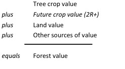
The purpose of this standard is to describe the method for establishing the market value of a forest or a tree crop. The distinction between these entities is based on the following terminology:
Standard B12.1 – Method of Valuation
In estimating the value of a forest or tree crop, the valuer shall consider the three most commonly recognised approaches:
- the sales comparison approach;
- the income approach; and
- the cost approach.
The valuer shall use their professional judgement in applying a credible weighting to each to produce an estimate of market value.
Should it be evident that one or more methods is of low relevance, the valuer may dispense with such method(s) in the interests of concentrating productive effort. It is nevertheless the valuer’s responsibility to explicitly declare where they have dispensed with the method(s) and provide their reasoning.
Given that the purpose of the exercise is to produce a market value, the valuer should attempt at all times to see the assets through the eyes of market participants. This encourages emulation of the methods by which such participants have arrived at agreed transaction values.
In estimating tree crop value and future crop value, the opportunity cost of land shall be included using market rental, regardless of land tenure.
If the land is leased there may be a land tenure differential when the actual land rent differs from the fair market rental. This land tenure differential shall be reported separately from crop value as the lessee’s interest in the land or the lessor’s interest in the crop (as the case may be).
In estimating forest value (or the value of a bundle of assets including tree crop value), the valuer shall ensure that there is compatibility in how the values of the different components have been estimated.
Among the distinctive features of forest valuation, the following may especially influence the result. The valuer must accordingly document their assumptions in relation to:
- the number of rotations recognised in the cashflows on which the valuation is based;
- identification of whether tree growing is considered compatible with the highest and best use of the land;
- the land value/tree crop value interrelationship – this includes confirmation of consistent assumptions in valuing the land and trees;
- treatment of forest roads and other durable assets; and
- whether the modelling of the forest is estate-based or stand based.
The valuation approach can potentially be either estate-based or stand-based. However, in both cases there needs to be an underlying management and harvesting strategy which is realistic for the forest (or tree crop) being valued. This strategy should reflect what an ‘economically rational’ owner would do taking into account wood supply commitments as well as logistical, marketing, social, political and environmental factors. The need to include these factors means that, in practice, a stand-based approach is only suitable for small forests.
GUIDANCE NOTES ON THE VALUATION METHOD FOR FORESTS OR TREE CROPS
Terminology
The standard begins with a terminological framework. This identifies the forest value as comprising the values of the tree crop, the value of future tree crops (2R+), the value of the land occupied by the trees* and values attributable to other components (e.g. carbon). Note that this is a simplified representation.
The point of the classification is to reinforce the role of assigning ‘forest value’. The professionals to whom these standards are primarily directed could conceivably keep their brief simpler and less demanding by just attributing a value to the tree crop (and future crop value). To this could then be added an estimate from a land valuer, conceivably providing the total forest value. Experience has confirmed that unless one valuer takes responsibility for combining the parts, the process is readily capable of producing an incoherent result. To ensure (as required by this standard) compatibility, one party will need to visibly assume the duty of ensuring additivity. Without this, the respective parties should document their individual responsibility for contributing to the valuation of a forest.
*Land tenure circumstances may commonly lead to a distinction between the freehold value of the land versus the value of an entitlement to occupy the land. This distinction is addressed later in these Guidance Notes.
Market value as the target
The focus of this standard is the estimation of the market value of a tree crop or forest or bundle of assets. In estimating market value the forest valuer is estimating the ‘amount of the cheque’ given by the purchaser to the seller. Selling costs are not deducted. This contrasts with financial reporting standard IAS 41, which requires a forest asset to be measured at its fair value less costs to sell.
Discounted cash flow analysis
Forestry characteristically involves long investment timeframes. Discounted Cash Flow (DCF) analysis is correspondingly pervasive. In other types of asset valuation, the application of DCF is commonly treated as synonymous with the income approach. Forest valuers may be more inclined to apply DCF methods within each of the three common approaches. Thus:
- the income approach explicitly applies a DCF methodology in accordance with its expressed definition; in applying the sales comparison approach to forestry, it has become increasingly common to turn to the Implied Discount Rate (IDR) as the most convincing unit of comparison noting the IDR is inherently applied within a DCF framework; and
- when the cost approach is applied to forest valuation, it is generally proposed that the entitlement to a return on invested fund should be considered noting when incorporated in the form of notional compound interest, such a return is also an expression of DCF methodology.
One case where DCF is seemingly not applied is where the value of a tree crop is based on the currently realisable value of its standing content (a ‘standing stock’ approach). This still fits within a DCF framework by recognising that the discounting period is zero years.
A diagrammatic representation of the methods is shown in Figure 12-1. The figure acknowledges that opinion varies on the extent to which methods that employ IDR can be described as manifestations of sales comparison*. They are accordingly linked by dotted lines to both the sales comparison and income approaches.
Figure 12-1 also recognises that if compounding (the reverse of discounting) is applied to costs, the rate might come from a ‘first principles’ derivation or from IDRs. If the latter, this provides the case for a methodology that combines the principles of both the cost comparison and sales comparison.

Forest valuers are encouraged to avoid using such terms as DCF and Net Present Value (NPV) incautiously. Forestry’s multi-period investment profile means that all three primary methods may ultimately rely on a DCF framework. Loose reference to a ‘DCF approach’ or an ‘NPV approach’ may potentially mislead those from other areas of business practice where DCF analysis is confined to the income approach.
*There are some valuers who would argue that at any reference to ‘discount rate’, the associated process can only possibly be
an income approach. Others respond by questioning whether the IDR is truly a discount rate at all. It might just as readily be
called an Implied Discount Factor, they argue, providing a link between the derived cashflows for a transacted forest and its
sales price. Those of an inclusive disposition are encouraged by the observation of Ackerson (Ackerson, C. B. 2009.
Capitalization Theory and Techniques: Study Guide, Appraisal Institute) who suggests that, in practice, the three approaches
may be inextricably intertwined.
Common or distinct cashflows
A potential implication of a ubiquitous DCF framework is that all valuation approaches might be based on the same set of cashflows. This is not axiomatic. The analytical procedures may be sufficiently distinct that differences extend beyond a difference in discount rate selection to a difference in cashflow derivation as well. At first impression it could appear unlikely that more than one system of cashflow projection could or should prevail. In practice, there are several reasons including:
- the treatment of risk in the cashflows;
- the duration of the cashflow projections;
- whether the cashflows are pre- or post-tax; and
- how the cashflows acknowledge debt-leveraging effects.
A Weighted Average Cost of Capital (WACC)-based approach typically employs the Capital Asset Pricing Model (CAPM) as the basis for estimating the cost of equity. It is the textbook recommendation that while the CAPM formulation implicitly acknowledges certain types of risk, the discount rate should not be regarded as a catch-all location for a whole basket of risk factors. It is technically better practice to factor certain types of risk into the projected cashflows to which the discount rate is applied. Indeed, the empirical market evidence on which key inputs to the WACC/CAPM is based may be effectively predicated on an expectation that cashflow projections are risk-adjusted.
Forest valuers are not observed to apply much sophistication in risk adjusting the cashflows. One influential reason may rest with practical difficulties. However, provided the forests being compared have generally similar risk characteristics, then the lack of cashflow adjustment need not disqualify an IDR procedure. IDRs can be extended from the referenced forests to the subject if the cashflows for all have been estimated on the same basis.
On the basis of risk treatment, two forms of discount rate may co-exist, each with a corresponding form of cashflow:
- WACC/CAPM rate, to be used in conjunction with risk-adjusted cashflows; and
- IDR, to be used with conventionally represented cashflows.
It is therefore possible to have IDR and WACC/CAPM estimates of the discount rate that differ without them being contradictory.
Market valuation versus client valuation
Market value is the amount for which the tree crop or forest should exchange:
- on the date of the valuation;
- between a willing buyer and a willing seller;
- in an arm’s length transaction;
- after proper marketing; and
- wherein the parties had each acted knowledgeably, prudently and without compulsion.
The underlying benchmark of crop or forest valuation as defined here is the estimation of the market value. In applying DCF analysis, there needs to be an underlying management and harvesting strategy which is realistic for the tree crop or forest being valued. This strategy should reflect what an ‘economically rational’ owner would do taking into account wood supply commitments as well as logistical, marketing, social, political and environmental factors. The appropriate ‘client’ valuation for a particular situation will depend on the circumstances, but any departure from the underlying market value conventions should be noted. The client valuation (or valuation for intended purpose) may differ from this estimate of market valuation because of certain factors which relate to the circumstances of the particular situation and the purpose of the valuation.
For example, the client may require:
- a valuation which assumes managing a forest with five years of planting for a non-declining yield over a 30-year rotation;
- a valuation based on a rotation length which is a significant departure from the optimum;
- a valuation as a seller or a buyer of a forest, using a set of inputs specific to the client, in order to commence negotiations; or
- the client may be forced to sell the forest into an illiquid market.
When the client value differs from the market value, it is important that assumptions are stated, any departure from economic rationality is justified and sensitivity analysis is carried out. The client value should be presented as market value minus (or plus) the cost of incorporating economically irrational elements.
That is, market value (economically rational value or ‘highest and best’ value) should also be disclosed. The value for the current entity for the described purpose then represents the market value plus or minus a difference.
Market value ± market difference = value for purpose
The market difference can reflect factors such as:
- assumed management and harvesting for a particular owner;
- assumed supply commitments not covered by a binding contract;
- assumed price and discount rate; or
- a buyer’s discount or a seller’s premium (in the case of a sale).
Duration of the cashflows: current rotation versus perpetual
The financial reporting standards require:
IFRS13 fair value for Forest = Land value + Tree crop value
The immediately available reporting standards for the respective sub-components are IAS 16 (Property Plant & Equipment) and IAS 41 (Agriculture).
Financial reporting standard IAS 41 (Agriculture) covers the valuation of biological assets. Paragraph 22 states: ‘An entity does not include any cash flows for financing the assets, or re-establishing biological assets after harvest (e.g., the cost of replanting trees in a plantation forest after harvest)’*.
In the market, however, buyers are observed to be acquiring forests with every expectation that they will be perpetuating them. For larger resources, the ‘purchase models’ include long-term cashflows from multiple rotations. These are often derived on a levered post tax basis.
However, it is necessary to recognise that IAS 41 is not a standard for valuing forest assets – or at least not ‘forests’ as defined in these standards. IAS 41 is the standard that applies when reporting the value of the current tree crop within a forest. The fact that it is confined to the current tree crop is eminently sensible, given that IAS 41 is a standard for reporting biological assets. While a next tree crop may come to exist (and that prospect may have a value), such a tree crop is not alive (yet). Being alive is the defining characteristic of a biological asset.
IAS 41 has been widely misread to imply that forest valuations must be based on the current rotation, and yet that is not the case.
*It is noteworthy that IAS 41, along with its other IAS standards, is now on the verge of substantial adjustment. This arises with the introduction of IFRS 13 (Fair Value). The latter provides an umbrella statement on issues relating to valuation. Potentially contradictory or redundant references that had previously appeared in subsidiary standards are scheduled for removal. No change to paragraph 22 is proposed.
The contribution from 2R+
The requirement to observe IAS 41 has brought to the fore the value of the next and succeeding rotations (herein referred to as 2R+). Within some situations there will be no 2R+, or not at least belonging to the current investor. Tenure arrangements may see them exit the venture at the completion of the current rotation.
Should the investor continue, the raw results of a DCF-based analysis of 2R+ will generally produce a non-zero value. It may be positive or negative. Only in the exceptional circumstance that the Internal Rate of Return (IRR) of the next rotations exactly matches the discount rate would the NPV of 2R+ be zero.
Positive values
A positive value for the future rotations would clearly be encouraging, but market dynamics could render it temporary. If the valuer’s perception of the inputs to the calculation is matched by the market perception, then in an informed, rational and frictionless market, the upside should in due course migrate into the one scarce resource within the investment, which is the land. *
*For a discussion of the principles prepared in a New Zealand context see Turland, J. 1990. Quantifying the Effects of
Changing Log Prices on Land Values for Forest Valuations, New Zealand Journal of Forestry, 35(2): 22-26.
An increase in the price of the land (or the rent to use it) would then reduce the IRR of 2R+, bringing it back closer to the discount rate. The NPV of 2R+, which relates by definition to just the future tree crops, would ultimately be extinguished.
Although such a theoretical model is simple, it does not make reporting a positive value for future rotations straightforward. Cautious accountants and auditors can justifiably ask that if that is the way the market is meant to work, why has it not done so already? Why is the land valuer not ready to absorb the upside in land value?
The land valuer’s response could well be that the market evidence for land for planting is scant and difficult to interpret. Both tend to be the case. Without some activity and depth to the market they cannot propose that the tree crop valuer’s result is indeed an increment that could be classified as market value as opposed to just an investment value. *
*The definition of investment value identifies it as a value that might be perceived by a particular investor, but not necessarily
the value seen by the market as a whole.
Negative values
The application of a perpetual analysis may demonstrate a negative value (or lower return) being associated with future rotations.
An example situation is shown in Exhibit 12-1.

Possible pathways
These guidance notes suggest two possible procedures for those forests whose valuation models involve full or partial contributions from future rotation cashflows:
Procedure 1: Multiple rotation starting point
This case would be applied where the IDR is considered to best serve its role as a basis for comparison when expressed at the multiple rotation level.
1. As indicated in the table, a value for the tree crop has been based on cashflows which are modelled for multiple rotations. The contributions from the respective rotations (1R & 2R+) may be identifiable within internal analysis.
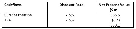
2. For reporting purposes and for assigning the cost of bush, the valuer calculates a discount rate at which the collective tree crop value corresponds to the NPV of just the current rotation cashflows.
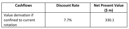
3. The sensitivity analysis accompanying the report should, for completeness, offer further examination.
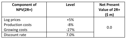
The first two tables facilitate the comparison of the multiple rotation discount rate with the single rotation equivalent that would provide the same value result. The comparison is a worthwhile form of disclosure.
The sensitivity analyses in the third table are for the purpose of testing whether a null hypothesis that 2R+ can ‘earn its keep’ can be rejected. It might emerge that only relatively small changes in single inputs, or a combination of inputs were required to bring the NPV(2R+) to a very low value. The valuer might then conclude that the contribution of 2R+ could be neutralised.
Procedure 2: Current rotation starting point
This case would be applied where the IDR is considered to best serve its role as a basis for comparison when expressed at the current rotation level.
1. In this case, the value for the tree crop has been based on just the cashflows arising from the current rotation. The 1R value of $330.1 million is reported in the Statement of Financial Position under Biological Assets (as per IAS 41).

2. The valuer should complete internal analysis, to calculate the single rate at which the same tree crop value may be obtained from multiple rotations.
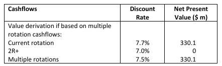
3. The sensitivity analysis accompanying the report should, for completeness, include further sensitivity analysis similar to that demonstrated in the previous procedure. These are shown in the table below:
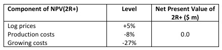
The third table is the same as that demonstrated in the multiple rotation IDR approach. The same type of sensitivity analysis as demonstrated in the earlier procedure could be used to demonstrate what change in variables would be necessary for the replanted resource to earn its keep. The breakeven rate in such analysis would be 7.7%, the discount rate associated with the current rotation model.
The emphasis of Procedure 2 is on reporting the return associated with the 2R+, as this is likely to be the metric that investors are most concerned with.
IFRS13 does place emphasis on two reporting matters:
- disclosure; and
- whether the current use of the assets represents a highest and best use.
A responsible appraiser should use these as a justification for examining the IRR that the 2R+ rotations are demonstrating. For the example resource the IRR associated with the 2R+ is 7.0%.
Poor NPV(2R+) results
Under any of the demonstrated procedures, the performance of 2R+ might seem so intractably bad that active steps are warranted to avoid re-investment. If there is a contractual obligation that compels the forest investor to plant subsequent rotations, the contribution of 2R+ might be reported as a liability, with the sum of the parts (asset value [reported under IAS 41] + liability [reported under IAS 37]) equating to net asset value. In the example given above this would be represented as AUD/NZD336.5 million [IAS 41] less AUD/NZD6.4 million [IAS 37], giving a net asset value of AUD/NZD330.1 million.
Positive NPV(2R+) results
Although the example provided above is for the situation of a negative NPV for 2R+, the same general procedures are applicable to the situation where the NPV for 2R+ is positive.
Meeting all the financial reporting standards
Either of the procedures provides a value for the tree crop that could appear within IAS 41 and IAS 37. If these values are added to the land value (reported under IAS 16), they should add to a market value for the forest (subject to including other applicable contributions from carbon etc). The resulting forest value should be consistent with general valuation standards, this forest valuation standard and the overarching financial reporting standard, IFRS 13 Fair Value.
Just as importantly, by addressing the procedures involved in the sensitivity analysis, the reporting is adhering to other requirements of IFRS 13 Fair Value.
Land value/tree crop value interrelationship
Separation of land and tree crop values.
Although, from a biological perspective, trees and land are inseparable, there are a number of reasons for partitioning forest value:
- land and trees are often owned by different parties;
- when an immature forest is sold in certain jurisdictions (including Australia and New Zealand) the components of value attributed to land and trees have different tax treatments;
- financial reporting standards also require a partitioning of value between land and trees; and
- separating the respective values is instructive in confirming that the land and tree crops are being managed according to best commercial interests.
Cost of land for tree crops
This standard requires that the opportunity cost should be calculated as the market-based land rent. Even if there is no rent for the land, there is no practical or conceptual obstacle to assigning a notional rent. The cashflow projections for the forest are appropriately parsed. Rather than occupying the land at no cost, the tree crop is charged a rent, and its value is accordingly reduced. The land asset receives the notional rent, and its value is correspondingly bolstered. If the rent is equivalent to market rental levels it might be proposed that the land’s market value can be sustained. There is accordingly no ‘encumbrance’.
The estimation of a market-based land rent requires consideration of the attributes of the specific piece of land and its alternative land uses. Market rent is the rental that might be expected to be paid:
- on the date of the valuation;
- between a willing lessee and a willing lessor;
- in an arm’s-length transaction;
- after proper marketing; and
- where the parties had acted knowledgeably, prudently and without compulsion.
A way in which the question can be most conveniently framed is, ‘What rent would result if land, in cutover state, was offered to the market?’
Note various Australian Government plantation privatisations involved the sale of the existing tree crop and the rights to use government land for a defined period for future tree crops, and no ongoing obligation to pay the titleholder of the land (i.e. the government) for the use of the land. In these examples, the purchase price included the access rights to the land to conduct forestry activities for existing and future tree crops. At present, common practice is that the market value is assumed to recognise the cash arising from the existing and future tree crops for the period remaining relating to the access right, inclusive of any value relating to the access right.
The better approach is to recognise the lessee’s interest in the land through a notional land holding cost (notional land rent), reportable under IFRS 16. Note the valuer will need to consider an appropriate representation of land value, land rental and expected discount rates to the land and tree crop, and the combined asset. In the event the land and tree crop cashflows are assumed to expect the same discount rate the net balance sheet difference between the two methods should be negligible, and the latter approach will provide a fairer representation of the economic reality of the situation, for example when tree crop values are compared to ‘similar’ tree crops on adjacent freehold or leasehold land.
Augmenting the Rent Database
The scarcity of pure market evidence for forest land rents does raise the question of whether other rent evidence has any possible relevance. It is suggested that grazing land rentals can usefully be introduced as a basis for comparison, provided that they are kept distinctly identified. They serve as a useful reference point on the basis that:
- they are empirical evidence;
- in Australia and New Zealand, broad acre grazing activity is arguably the closest counterpart to forestry in terms of competing land-use. If the rent levels were to be substantially different it would suggest that something was awry in the assembled evidence; and
- grazing rents can be expected to show some broadly similar behaviour to forest land rents in respect of several key site characteristics, including fertility and terrain.
If used to augment the forest land rental evidence, grazing rentals need to be adjusted to reflect land in a cutover state. Adjustments need to be made for factors such as:
- the presence of stumps;
- improvements; and
- the rental term.
The most appropriate grazing land rentals would be those of a long duration. In contrast, if grazing is being presented as a potential higher and better use (HBU), then whatever tenure term provides the highest returns can form a legitimate comparison.
Rent and tax
The land rental should be treated as being tax deductible when valuation is based on after-tax cashflows. It is assumed that the parties in the rental market set rentals with knowledge of the tax deductibility.
Worked example
The following page provides an example of using the land rental approach in valuing a tree crop. The example highlights the need for the forest valuer, in determining the market rental, to consult with the land valuer to ensure that there is consistency in the assessment of prevailing rentals and the determination of land market value.
Reconciliation with land-in/land-out approach
The land-in/land-out approach is an alternative approach for estimating the cost of land in the valuation of a tree crop. Land is assumed to have gone in at the starting year of the cashflow calculation (i.e. the starting year of the investment or the current year for a valuation) and come out at the end of the rotation. Discounting of the land value at the end of the rotation should be at the appropriate discount rate for land. The crop value generated can be reconciled with that produced using the land rental if an appropriate adjustment is made for land appreciation before the end of the rotation.

Forest on rental land rather than freehold land
The same basic principles apply for both freehold and rental land (whether a lease, licence or forestry right is involved).
On leasehold or in New Zealand the Crown Forest Licence (CFL) land the actual rentals paid should form the starting point in determining the market-based land rental. However, if these rentals are materially different from market rentals then separate analysis is required to calculate:
PV (open market rentals) = PV (actual rentals) ± land tenure differential
The PV of future obligations of rental payments below open market value represents the lessee’s implied interest in the land. Conversely, if the PV of rental payments on the leasehold land were above the open market value the difference would represent the lessor’s implied interest in the trees. *
Land tenure differential is institutionalised by the land occupation contract (e.g. lease, licence). To the extent that land tenure differential does not equal zero, the value will transfer from the lessor to lessee or vice versa. As it is a real transfer and recognised by the rights given to each party under the lease, it should be reported as the lessee’s interest in the land or the lessor’s interest in the trees.
* May need to consider cases in AU where, with the purchase of the asset, the land rental was paid up-front, that is the grower has ‘rent free’ use of the land.
Treatment of other durable assets
Subject to the below qualifications, other types of assets may also figure in an overall forestry venture. Examples include:
- improvements on the land including roads, bridges, fences and dams;
- buildings used as office premises, worker accommodation, equipment shelter and maintenance, and for storing chemicals;
- fire-fighting equipment; and
- mobile plant and equipment.
If such assets are already owned by the forest venture, then they potentially provide the benefit of an avoided future cost. For example:
- if a roading network already exists, future capital cost may be avoided;
- if a tractor and set of discs used in land preparation are already owned by the venture, then the projected cashflows do not have to make provision for their future hire or purchase; and
- if vehicles for transporting workers to the forest are already owned, the future outlay on buying or renting them is averted, at least until the end of their useful life.
The scale of these assets might be small and not material and they may already be covered as an overhead cost. Where material and not already covered, the valuation of these assets can be on the basis of avoided costs (see Standard B6).
In estimating the tree crop value using DCF the ongoing costs should be included. For example:
- in the case of roads, ongoing costs of maintenance costs should be included as well as the cost of upgrading existing roads or building new roads; and
- in the case of plant and equipment, ongoing operating costs of fuel, tyres, repairs and maintenance as well as capital costs to replace the equipment (offset by the salvage value of the equipment being replaced) should be included.
The cost of the existing asset should also be included in the cashflows. Two possible approaches for doing this are:
- value-in/value-out – the initial ‘value-in’ is the current value while the ‘value-out’ would be the depreciated value (such analysis needs to be run with the appropriate discount rate for the asset type); and
- notional rental – the tree crop should be charged with a notional rental based on the market rental or hire charge for the asset.
Care needs to be taken with depreciation. Generally, it should not be included as it is not a cash cost, but the tax effect of depreciation needs to be included if post-tax cashflows are modelled. In some cases, it may be included as a proxy for ongoing capital costs.
Estate modelling versus stand-based modelling
Forest estate models can be described as providing a ‘top-down’ approach to managing a resource. They simulate the behaviour of the collective forest resource at once, manipulating its woodflow, cashflow and other attributes within overall constraints. Because management of the collective estate is the target, the fate of individual stands is subservient.
In contrast, stand-based modelling effectively treats each stand in isolation, ignoring the extent to which its woodflow complements or supplements the output from others. The results from all the individual stands can then be summed together, providing a ‘bottom-up’ approach.
There have been attempts to develop estate models within spreadsheets, but these have generally not provided an adequately compact and efficient structure. For larger resources, appraisers turn to purpose-built software. Within Australia and New Zealand, the pioneering packages dominant from the mid 1980s were RMS2020 and FOLPI. At the time of writing, two of the state-of-the-art packages are Woodstock and Tigermoth.
As a general rule, valuations based on forest estate modelling will provide a lower value than those derived from stand-based modelling. The explanation lies with the concept of the optimum economic rotation age. In principle, this age is the one at which the marginal rate of value growth matches the discount rate. It is at this age that the NPV of the stand is maximised. Felling the stand either earlier or later results in a lower NPV.
The distinguishing feature of forest estate models is their capacity to vary the age of harvesting in order to manage the woodflow and cashflow profiles. The constraints that estate models impose will inherently lead to departures from the optimum rotation age and they correspondingly result in a reduction in value. However, if the forest estate model constraints are realistic this version of the forest value is more authoritative. The stand-based alternative can be treated as an interesting but impractical ideal. An estate model version of the forest can be regarded as the general and most realistic basis for valuation. Situations involving small or simplified forests that can be modelled on a stand basis represent special cases. The default position, therefore, is that the forest should be modelled as an estate and an explanation provided if this is not considered necessary.
Disaggregating the estate model
Within a stand-based model it may be amply clear which costs are incurred in generating which ultimate revenues. Each is readily itemised at the stand level and can be apparent before any process of aggregation. With forest estate-based models, the typical cashflow output is aggregated to an extent that masks which costs relate to which revenues. A simplified example of the effect is illustrated in Figure 12-2.
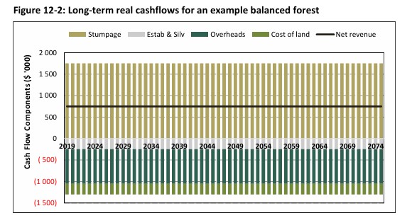
A financial analyst examining Figure 12-2 might conclude that engagement in forestry is an especially desirable type of business. The net revenue profile for the project shows an endless positive margin, so whatever the discount rate employed, the NPV remains positive. On closer examination, however, it is apparent that many of the costs incurred in any year do not relate to the revenues obtained in that same year. The establishment costs, for instance, are not recovered until the end of the rotation.
If the cashflow shown in Figure 12-2 was to be parsed into the components attributable to the current rotation and 2R+, these might look like those shown in Figure 12-3. Now it emerges that 2R+ will have a negative value at all discount rates that exceed the constituent stands’ IRRs. *
*The IRRs that apply at the stands’ harvest ages as constrained by the estate model.
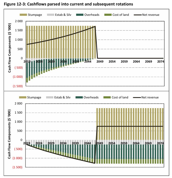
Given the capacity of the aggregated cashflows to mask the underlying investment performance of the resource, it is best practice to distinctly identify the contributions from the current rotations and those that follow. The available software packages support this capability.
Valuing different types of plantation forest
Within the emphasis being given to assessment of fair value, practitioners are advised to emulate the processes followed by buyers and sellers. The practices are seen to vary, depending on forest size and age-class distribution.
Small forests, confined age class distribution, old
Primary attention is given to standing stock valuations. To rigorous vendors and purchasers there is justification in testing the hold or sell decision, which leads to the application of DCF-based concepts.
Small forests, confined age class distribution, young
Primary attention may be given to a cost-based approach, but there is also a need to confirm future viability and this invokes the discounting approaches. There is, therefore, a role for DCF based concepts in both discounting the future projected revenue stream and in assigning accumulated returns on investment.
Small forests, confined age class distribution, mid-rotation
Such forests are uncommonly traded for a combination of reasons. In the absence of comparable sales evidence this leads to a heavy emphasis on the income approach. There may need to be an added overlay recognising the thin nature of the market and the lack of debt finance.
Medium forests, some spread to age class distribution, but predominantly young
Such forests are less commonly traded because of the delay in receiving sizeable cashflows and limitations on debt servicing capability. The main emphasis is on discounting approaches and reference is made to comparable sales wherever these are evident. There may need to be an added overlay recognising the thin nature of the market and the lack of third party debt finance.
Medium forests, some spread to age class distribution, and with a significant component at and approaching harvest age
Valuation of these is likely to involve DCF approaches that reference both the IDR (sales comparison approach) and the WACC (income approach). The forests may be beneath the value threshold at which TIMOs will engage and this needs to be considered in addressing the universe of potential buyers.
Big forests, distributed age class distribution
At the time of writing this class of forest is of interest to TIMOs, other institutional investors and industrial interests. Purchasers may fund part of the purchase price from debt to obtain leverage benefits. The financial models that the purchasers and their advisors apply in deriving their bid values involve multi-rotation, post-tax, post-leverage cashflows.
Despite the increasing sophistication of the purchase models, there is still a legacy of reporting of market evidence based on single rotation and/or pre-tax cashflow models. If forest valuers are to adequately emulate market practice, they will be required to produce the following versions of the valuation model:
- current rotation model;
- perpetual model; and
- purchase model.
All versions must be reconciled to the same value result.
GUIDANCE NOTES ON YOUNG FORESTS
Young forests
When valuation discount rates are higher than the Internal Rate of Return (IRR), the expectation value approach can give unrealistically low (including negative) ‘values’. Conversely, when discount rates are lower than the IRR, unrealistically high ‘values’ may be derived. In such cases, an approach to valuation that includes consideration of replacement cost is necessary.
The small amount of transaction evidence on young forests indicates that, in some cases, the sellers are satisfied with getting their development costs (‘replacement cost’) back. Further, they may be willing to recover only the direct costs incurred (i.e. excluding indirect costs and land use costs with or without compounding).
Where a young forest is valued periodically (say annually) over a number of years (during which time it becomes an ‘old’ forest), the valuer can expect a discontinuity in value if they switch from 100% reliance on current replacement cost method to 100% reliance on the expectation value method at a fixed age.
If transaction evidence were to support the view that market value jumps up or down at a specific age, because buyers and sellers are want to switch their view of value at that age, then a discontinuity is justifiable. Otherwise, and this is more likely the case, a discontinuity is symptomatic of incomplete consideration of the weights that should be given to expectation value and current replacement cost and how those weights change with age.
Some valuers progressively increase the weight given to expectation value evidence and decrease the weight given to current replacement cost evidence as age increases, in order to reduce the likelihood of a discontinuity in valuations. Such an approach is acceptable.
The key requirement of a forest valuation is that it passes the reality test, i.e. is the value struck likely to result in a transaction (should the forest actually be marketed) given all the evidence available to the valuer?
Consistency
An important consideration is one of consistency. If a subset of stands in a large forest were to be valued on a stand-alone basis, would the value be similar to the apparent value of those same stands when valued as part of the large forest?
The scope for inconsistency of values exists, particularly where different valuation methodologies may be applied, depending on the disposition of the subset of stands. Particular care is therefore required in valuing young stands.
The potential for arbitrage may exist where forests are valued and exchange hands, with the subsequent on-sale of a subset of stands. It may not be necessary to avoid the potential for arbitrage, but the valuer should be aware of its existence and draw the client’s attention to it.
Forests with bi-modal age structure
Some forests comprise near-mature stands and young stands with no or few stands of intermediate age. They can arise when a forest established over just a few years reaches maturity, harvesting commences, and young stands start to appear as replanting proceeds. These forests thus comprise a ‘young forest’ and an older forest. Applying the income approach alone to such a forest may result in an unrealistic assessment of value.
An appropriate valuation approach may be to value the young stands as a young forest and to value the older stands using a method appropriate to those stands (i.e. income approach).
The test to apply is: ‘Is a potential purchaser likely to regard the forest as essentially two forests, each valued using a different method? Is the value struck likely to result in a transaction?’
A wide range of forest age class structures is present in the national estate, and it is constantly changing. A particular instance has been described, and a wide range of variations exist around it. In some cases, a particular judgement call will be required as to the best approach to valuing a subject forest with such an age structure.
Young forest taxation effects
When valuing young forests, the taxation situations of both the owner and the hypothetical buyer will need to be considered. The following example shows that taxation effects can create a gap in value expectations between seller and buyer.
Example
Seller spends $100 developing a young forest
Seller earns tax deductions of $33
Net outlay of seller is $67
Seller wants to recoup net outlay upon the sale of the forest
Seller is taxed on the proceeds from the sale
Seller therefore wants to sell at: $100
Buyer has to place purchase value in a cost-of-bush account
Buyer therefore has no immediate tax relief
Buyer has the option of developing its own young forest at a net outlay of $67
Buyer expects to purchase the forest for: $67
Aspects of applying the compounding approach
The application of the compounding approach invites questions about how the following should be treated:
- compounding rate;
- direct cost assumptions;
- assumed overhead costs;
- land cost; and
- taxation.
A generally observed feature of the method is the application of a comparatively low rate of compounding. This is believed to primarily reflect the concern that undue reliance on compounding can lead to a high-cost forest being valued more highly than it should. Valuers are aware that forests that are expensive to establish may not be ultimately the most productive.
The acknowledgement of this concern results in the selection of compounding rates that are less than the discount rate. Some valuers indicate that when considering a compounding rate, they also perform a cross-check and calculate the Internal Rate of Return (IRR). Their premise is that it would be unreasonable for a value produced by compounding to rise at a faster rate than the IRR.
Generally observed compounding procedures use direct costs and overhead costs that are at industry-standard levels and are consistent with achieving a forest of the standard represented. The costs are expressed in current-day values. In this respect, the value obtained by compounding differs from the accumulated book value that may appear in accounting reporting (as described in Section A3). The latter is more likely to use historic actual costs, with no indexing to adjust for inflation.
By and large the compounding process is meant to provide the reverse procedure to discounting. Consistency suggests that there is recognition of land use charges, whether actual or notional.
Application of professional judgement
The adjustments do rely on the valuer applying their professional opinion but are not without some rationale. At all times the guiding principle is to picture a hypothetical negotiation between buyer and seller and attempt to consider how the two parties would offer and counteroffer.
Factors to consider include:
- the tax position of the two parties (see above);
- that the seller’s perception of value is likely to be driven by what has been spent on the forest;
- the sum of direct costs incurred is likely to shape the seller’s ‘reserve price’;
- there may be more latitude over compensation for overhead costs, the cost of the crop using the land and the time cost of money;
- buyers are likely to be influenced by what it would cost THEM to develop a replacement crop rather than what it cost the seller to develop the crop being valued;
- buyers may argue that they could develop a replacement crop that was better through improved genetics or establishment practices;
- the seller might counter that because the trees are already in the ground there is less risk to a buyer and in addition, the rotation is already advanced.
GUIDANCE NOTES ON OTHER FOREST REVENUES
Introduction
Other Forest Revenues (OFR) relate to outputs from the forest, other than logs, that have economic value. They should be considered with the forest valuation and included where they are material and meet certain criteria. In certain circumstances, the OFR should be the subject of a separate valuation by the forest valuer or an appropriate specialist.
Examples of Other Forest Revenues (OFRs)
Outputs from the forest that fall into OFR may include:
- grazing;
- recreation;
- hunting;
- nectar;
- berries;
- fungi;
- honey and other apiary products;
- nuts;
- understorey vegetation;
- carbon sink capacity; and
- water catchment.
This list is not exhaustive.
Inclusion of OFRs
The revenue generated by these outputs that can be directly associated with the forest can be considered in the forest valuation. OFRs often tend towards social values. To qualify for an assignment of market value three criteria need to be met:
- Measurability
Measurement of market value needs to be based on the expectation of a future cashflow. The expected future cashflow stream should be based on current transactions arising from the subject forest or like forests. - Certainty
OFR may be uncertain or subject to extreme seasonal, year-to-year, or crop age dependent fluctuations, so appropriate conservatism is especially important. - Beneficial interest
The forest grower must have the right to benefit from the OFR.
Treatment of cashflows
The scale and nature of the OFR will indicate the appropriate treatment in the valuation process. Broadly, the two possible treatments may be characterised as the ‘separate enterprise’ approach and the ‘bundled’ approach.
If the Net Present Value (NPV) of the OFR exceeds about 5%* of the present value of the future cashflow of the tree-growing enterprise, the former approach is indicated. The approach selected requires a judgement call of materiality and utility and the valuer should consider these factors (as well as scale) in making it:
- is the venture inextricably associated with the presence of the tree crop? (if so, a bundled approach is required);
- is the venture able to be carried on through the whole rotation? (bundled);
- is the capital and management best provided by the forest owner? (bundled);
- are the costs joint with other forest operations? (bundled);
- is the venture amenable to legal separation? (consider the potential to separate);
- are the OFRs a necessary part of the economics of the forest enterprise? (probably separate but a bundled analysis may be required if a failure of the OFR will have a crucial effect on the forest enterprise and hence its value or vice versa);
- is the venture in the subject forest actually a separate enterprise at the date of valuation and the rules of separation nullifies the management of one enterprise affecting the other? (separate);
- is the continuation of the OFR venture discretionary to the forest management? (bundled);
- is the continuation of the forest venture discretionary to the OFR management? (separate);
- does the venture provide values to the forest that are difficult to quantify and isolate such as public relations benefits, staff interest, soil fertility? (bundled); and
- are the costs and revenues relatively certain and continuous, and would a prudent person undertake a business venture based on them? (separate).
*Indicative measure of materiality.
Separate enterprise
The separate enterprise approach presumes the existence of two business opportunities and requires the separation of all costs and revenues between the forest and the OFR business.
Appropriate arms-length transaction values for services and assets provided by each business to the other will be derived and used in each valuation. A valuation for each business will be derived from the separate cost and value streams. The enterprises may be valued with different discount rates and/or funding assumptions.
If the business of the OFR is outside of the competence of the forest valuer, and particularly where legal commitment to it is required, its valuation will require outside assistance. An example of the treatment of land rent, which is a typical transaction between a forest and a separate enterprise OFR, is shown below.
If the OFR actually pays (or alternatively can on reasonable grounds be imputed to pay) a rent to the land, this can be considered a value of the OFR to the forest enterprise and reported separately. In the sum of both enterprises the rent will cancel out.
If costs not allocated to the OFR fall on the forest venture (say skinning of trees by trail riders), the unallocated costs are best viewed as a forest cost borne to achieve an outside income (rent) to the forest.
If the forest business and the OFR business are in one ownership, the decision to continue with the OFR business rests on the worth of it less/plus any unallocated costs/benefits identified and valued in the forest business. The separate business (and the value effects on the forest) are assumed sheddable by the land /forest owner’s decision. If there is separate ownership or legal commitments (either way) between the forest business and the OFR business, the decision is subject to these and can only be exercised when the commitments have expired or are to be reviewed.
Bundled
No appreciation of the separable value of the OFR business is directly indicated by the bundled approach. The stance is that small items of cost and revenue are inextricably part of the forest enterprise.
The effect of the OFR is expressed as the costs and negative costs of growing trees on that site and is subject to management control in the ordinary course of the forest business. Continuation of the OFR business is discretionary to forest management. It is of small importance to the success of the tree crop or the economics of the whole venture and may be regarded as a ‘by-product’.
Example
The example below assumes a true arms-length relationship between the forest owner and the proprietor of the OFR, i.e. a separate enterprise.
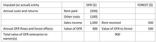
OFR land not separable from forest land
In the foregoing example neither the forest owner nor the OFR proprietor would wish to discontinue their respective enterprises. However, this assumes that the forest owner does not allocate a land-holding cost to the OFR enterprise area.
This assumption is consistent with an assumption that land ownership cannot be shed from the forest enterprise to the OFR business. The forest enterprise bears the ownership cost of the land because there are no other options for the main business and this business is not affected by the existence or otherwise of the OFR.
Say the allocated holding cost of the unsheddable land asset is $600 per annum. The complete value statement for the landowner is that he or she bears unsheddable costs of $600 but is able to gain a return of $500 by also using the land for the OFR business.
OFR land separable from forest land
If the OFR land is separable from the forest land, then the landowner is justified in allocating a land-holding cost:
Say sheddable land-holding cost ( 600 )
Rent from OFR 500
Net value of OFR to landowner ( 100 )
If the landowner does not own the OFR business, the logical course is to sell the land at any price greater than capitalising $500 at the forest discount rate.
If the landowner also owns the OFR, the decision to sell the land and the OFR business rests on the sum of annual income ($900). This indicates the landowner would keep the OFR business and the land if the price obtainable for the land and business is less than $900 annual income capitalised at the discount rate of the OFR business.
GUIDANCE NOTES ON FOREST VALUATION CONVENTIONS
Purpose of conventions
A valuation is a communication based on an underlying calculation. Any calculation and communication require consistent conventions to control the information and the process. The conventions adopted must also meet the needs of the recipient.
There is clearly little utility in a valuation having an internal crop age convention different to the age conventions applied to the yield table and the discount intervals. Neither is there utility in presenting a valuation with an internally consistent set of conventions that does not match the realities of the client’s position. For example, stumpage values applicable to a large corporate forest owner when the client has a small forest remote from markets. There are many possible, and valid, internally and externally consistent convention sets for any one valuation. The following set is designed to be consistent with the abbreviations and definitions set out in the Glossary. Its use will help to limit the number of differences between valuations.
Some of the conventions may seem surprising and pedantic, but they are nevertheless consistent with widely accepted valuation treatments and are necessary.
Disclosure of conventions
The convention set outlined in these Guidance Notes is recommended for adoption (but is not mandatory).
The valuation document should include a note of the convention standard adopted.
[This valuation uses the standard set of conventions as recommended by Forestry Australia or New Zealand Institute of Forestry] or [This valuation uses the standard set of conventions prepared by YYYY as described in Appendix Z.]
The most appropriate place to make this disclosure is in the ‘Method’ section of the valuation.
Definitions
Refer to Chapter E2, Glossary of Forest Economic Terms for definitions of:
- valuation event; and
- discount point.
Time conventions
General conventions:
T1G Even though time is continuous, valuation events are deemed to occur at, and statistics are recorded at, discrete instants.
Specific convention (example):
T1S The valuation year runs from 1 July 20X1 to 30 June 20X2.
T2S A stand experiences its annual growth increment (yield indicated at age B minus yield indicated at age A) at 11pm on 30 June. Yield tables are indexed so that ‘Yield at Age 17’ indicates the yield at the 17th birthday (including the increment over the immediately previous year all notionally added at 11.00pm on its 17th birthday).
T3S Age – seedlings and cuttings are deemed to begin life (age 0) on 30 June of the calendar year of planting. A stand has its birthday at 11.30pm on 30 June. Implication: All trees planted in calendar year 20X1 are aged 0 until 11.30pm on 30 June 20X2 when they become age 1.
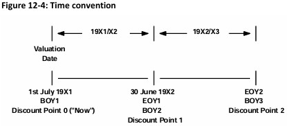
T4S The discount point in year 20X1/X2 is at 12.00pm on 30 June 20X2.
T5S 12.00pm (midnight) on 30 June 20X1 is the Beginning Of Year (‘BOY’) 1 or point 0 in a discounted cashflow. 12.00pm on 30 June 20X2 is BOY 2 and End Of Year (‘EOY’) 1 or point 1 in a discounted cashflow.
T6S A value stated to be ‘at 20X1’ is at 12.00pm on 30 June 20X1.
Implications:
− A valuation required to be placed at 31 December 20X1 will be initially made as at 12.00pm on 30 June 20X1. Any valuation events that actually occurred between this time and 31 December 20X1 (i.e. possibly some 20X1/X2 scheduled operations) will be adjusted at cost (or return). Interest and discount on the investment at 12.00pm on 30 June can be adjusted to 31 December if required. Adjustments may be made for reductions in stocked area due to clearfelling or other reasons (e.g. fire, wind loss). An adjustment may also be made for any volume increment/decrement after 30 June 20X1; and
− A stand aged 17 as at 30 June 20X1 will not have had ‘age 17’ costs expended on it (see specific conventions T7S). T7S Operations with costs or revenues described as taking place in valuation year 20X1/X2 take place at 12.30am on 1 July 20X1.
Implications:
− A valuation event in 20X1/X2 will not be discounted.
− A valuation event in 20X2/X3 will be discounted one year to 12.00pm on 30 June 20X1.
− ‘Operation at Age 17’ means ‘operations carried out while the tree is aged 17 years and before it is aged 18 years’.
− Note that other convention sets may assume operations occur at mid-year or end-of-year rather than at start-of year.
Note 1
For ease of explanation the conventions are expressed as examples, and the conventions apply similarly at all ages and years.
Note 2
Hours of the day are adopted for convenience to indicate the sequence of events.
The Figure 12-4 below illustrates the use of the above convention set.
Cost conventions
General conventions:
C1G The accounting rules applicable to the calculation of costs as promulgated by the Chartered Accountants Australia and New Zealand will apply.
Specific conventions:
C1S Future operations and their associated costs included in a market valuation are those that on the evidence available at the time are likely to add value to the existing forest at the chosen discount rate.
Implication:
− The costs included in a market valuation are to be those that an economically rational investor would apply to an existing forest to maximise its NPV. Valuations undertaken for different purposes may use a different convention with the reason for the departure explained (e.g. the conscious decision of the owner to grow the forest for mainly pulpwood production).
C2S Operational costs are at levels likely to be achieved by a competent manager of the subject forest operating at arms length from the forest owner. Costs shall be those that apply at the date of the valuation on ruling terms of trade from contractors skilled in the operation and operating in the area of the forest.
Implication:
− A contractor’s overhead may be assumed to contain a travel time/cost component appropriate to the subject forest.
C3S All costs associated with valuation events are expended at the same time as the scheduled valuation event, along with all owner’s overheads associated with them.
Implication:
− Even though non-operational costs (such as administration charges) are continuous through the year, they are regarded as associated with a valuation event and timed accordingly.
C4S Tax deductions/liabilities associated with expenditure and income fall due at the same time as the associated cost/revenue. (NB: This is a conservative convention for most valuations).
Area conventions
General conventions:
C1G True area means the area as stated on a Certificate of Title, survey plan, block sheet or other plan prepared by a registered surveyor.
Specific conventions:
C1S Tree area of the stand in terms of ‘stocked hectares’ is the area occupied by tree canopy to the outside edge of the crown and excludes:
a) each canopy gap of more than one-tenth of a hectare within the stand boundary; and
b) all roads and service areas outside the tree canopy boundary.
Market conventions
Specific conventions:
M1S Prices for logs/stumpage/cutting rights are at levels likely to be achieved at the time of maturity:
- by a competent sales agent;
- at arms length;
- using ruling terms of trade;
- in the available and practical market(s);
- to give the highest total net stumpage; and
for the on-truck outturn indicated.
M2S Prices are to be converted to the net stumpage available to the forest owner.
Implications:
− all selling costs, costs between the stump and the applicable price point, and marketing costs and commissions are to be netted off the buyer price;
− the applicable quantity for pricing is ‘on-truck’ with realistic allowances made for unmerchantable produce, breakage etc deducted from the indicated yield table outturn; and
− the market price applied is not necessarily that to give the highest theoretical stumpage but the highest practicable return. It is not likely in practice, for example, that a small parcel of logs would achieve the same stumpage as indicated by export prices paid for large continuous supplies of similar specifications, even with all the costs applicable to the subject forest netted off.
M3S Prices are valid as at 30 June 20X1. (This convention requires a statement in each valuation.)
Discount rate conventions
General conventions:
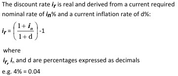
D1G:
D2G The discount rate is applicable to post-tax cashflows.
Last date updated: 31/07/2025